Edge, Corner, and Blob Detection
Canny Edge Detector (50%)
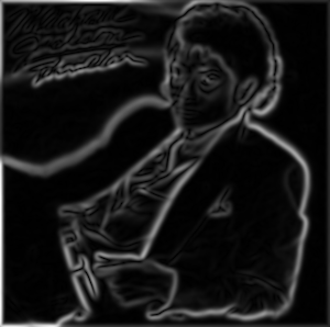
The canny edge detector is a robust edge detection algorithm that outputs thinned edge images while minimizing the impact from noise. I will use this image to demonstrate the different intermediate steps in the edge detection pipeline: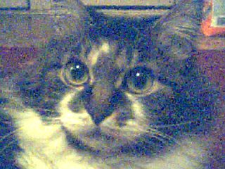
Algorithm Steps
Convert to grayscale and normalize to the range [0, 1]
Filtered Gradient
The goal is to compute the x and y components of the gradient, Fx and Fy, respectively. This could be done with a simple convolution kernel such as [1 0 -1] oriented along the x and y axis, but this method would be extremely sensitive to noise. Therefore, instead, it would be good practice to first apply a lowpass filter to the image, and then to take the gradient in the appropriate directions.
A good choice for a lowpass filter would be a Gaussian. Since its Fourier Transform is also a Gaussian, this means that it is compact in frequency space and drops off quickly enough to de-emphasize high frequency noise. Note also that the variance of the gaussian in frequency space is inversely proportional to the variance in the time domain. This means that the wider the gaussian is in pixel-space, the skinnier it is in 2D frequency space, meaning that a wider Gaussian decimates more high frequency components and leads to blurrier images.
Start with the following Gaussian filter, which has width sigma
\[ F(x, y) = \frac{1}{2\pi\sigma^2} e^{\frac{ -(x^2 + y^2)}{2\sigma^2}} \]
Then compose that operation with the partial derivative in each the x and y directions. This way, the suppression of noise can occur simultaneously with calculating the gradient
\[ F_x(x, y) = \frac{ -x}{2\pi\sigma^2} e^{\frac{ -(x^2 + y^2)}{2\sigma^2}} \]
Note that this expression is separable; that is, it can be decomposed into parts that depend only on x, and parts that depend only on y:
\[ F_x(x, y) = (\frac{ -x}{2\pi\sigma^2} e^{\frac{ -x^2 }{2\sigma^2}}) * e^{\frac{ -y^2 }{2\sigma^2}} \]
So applying this dual operation of noise filtering and partial derivative in one direction can be accomplised with two 1-Dimensional convolutions; one which is simply a gaussian, and the other which is x*the gaussian. This is much faster computationally than attempting to convolve with the 2-dimensional kernel Fx(x, y).
In practice, here's what I do:
I sample a 1D Gaussian of the equation:
\[ e^{\frac{ -x^2 }{2\sigma^2}} \]
..and one of the equation:
\[ -xe^{\frac{ -x^2 }{2\sigma^2}} \]
...where x ranges from -3*sigma to 3*sigma, rounded to the nearest integer pixel, for some chosen sigma. But note that the samples of the first equation do not necessarily sum to 1, which is necessary to maintain the average energy over the image. Therefore, after sampling the first gaussian, I scale it by 1 over the sum of its samples.
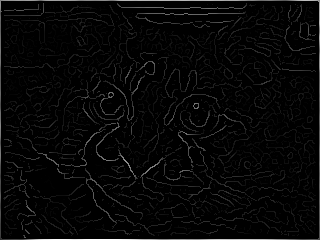
A similar problem occurs with the second gaussian with the -x coefficient in front (that results from taking the derivative). The goal applying that gaussian is to approximate a tempered derivative at every point. So it is expected that applying that kernel to an image that has a constant slope of, say, 1, should yield an output that is 1 everywhere. But it may not since I'm taking a finite sampling of it (and I completely ignored the leading coefficient). To put this into code, I create a ramp region that has a slope of 1, convolve it with this kernel, and determine the value. I then divide the kernel by this value so that applying it again would give 1 as the answer. Now I have all of the information I need to approximate the properly-normalized discrete intensity gradient of an image. Here are the results of convolving the gradient of this gaussian with sigma=2 to the example cat (NOTE: The gradient components are scaled so that they occupy an intensity region [0, 255], so that a higher contrast is visible. The actual values of the gradient are much weaker):
Input image
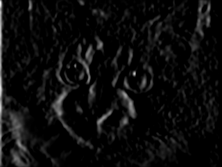
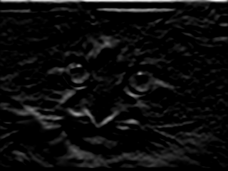
Fx Fy Magnitude of F Nonmaximum Suppression
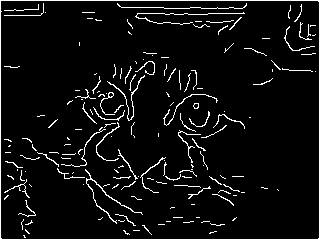
The process above seemed to work pretty well at detecting the edges, at least initially. But note that the edges are a bit blurred; there's a gradual transition from the beginning of the edge to the end, and the edges are all several pixels wide. What would be nice would be to extract a thinned edge image, where each edge is roughly only one pixel wide, and encompasses the strongest locations of each blurred ege. This is where this technique of nonmaximum suppression comes in.
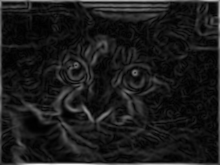
To accomplish this edge-thinning task, first compute the direction of the filtered gradient (from the previous step) by taking tan-1(Fy/Fx). Quantize this to the directions (0, 45, 90, 135, and their opposite angles 180 degrees off), as these are the only directions to get from one pixel to an adjacent pixel. Follow the direction of the gradient both forward and backward, and only keep this value of the gradient if it is greater than both of its neighbors. This will ensure only the strongest 1-pixel-wide part of an edge transition is kept. Here is the result of applying this operation:
Magnitude of F Nonmax Suppression Hysteresis Thresholding
Now the process is almost done. All that remains is to set a threshold on which edges are strong enough to keep, and which ones should be discounted. It would be possible to do this by setting one threshold and throwing out everything below that threshold. However, this is not very robust to noise in the intensity of the thinned edges. If there happens to be a slight variation in a thinned edge below and above that theshold, then the edge will come out disconnected in the final image. So what's better is to use two thresholds; one to choose an intensity value that the edge must reach at least once, and another to set a minimum intensity value of all points that can be in a connected region of an edge.
Note that to look at connected regions of edges, simply look along the level sets defined by the direction of the gradient; that is, the level sets that constitute the thinned edges, lie perpendicular to the gradient.
NOTE: I implemented this section recursively; that is, I found a point above the high threshold, and then recursively connected it to its neighbors along the low threshold. Apparently, matlab has a stack size limit of 500 for recursive functions. I found this out the hard way, since I usually have an edge that borders around my entire image due to zero padding during the filter stage. Since it's rare that an edge will be more than 500 pixels long if it's not on the border (as I mentioned), it's safe to just kill the recursion if it gets close to the limit (I set the limit to 450 in my program). Chances are that will just break up the edge along the border, which isn't that important (since it's not even supposed to be there anyway)
Here is an example of the final product throwing everything together with thresholding:
Nonmax Suppression Final Output Image Automatic Thresholding (Optional)
As an optional last step, some algorithm can be used to automatically generate the thresholds used in the previous step. I came up with the following simple algorithm to generate the thresholds:
- Take the average of all of the pixels remaining in the thinned edge image
- Set the high threshold equal to the average of all pixels above this average
- Set the low threshold equal to the average of all pixels below this average
Results of varying different parameters
Syntax: Canny(filename, sigma, high_threshold, low_threshold, filenameout)
NOTE: If the high_threshold is set to zero, then thresholds for T_l and T_h are chosen automaticallyClick on the hyperlinks to see all of the intermediate results for each command
-
Varying sigma
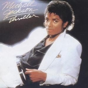
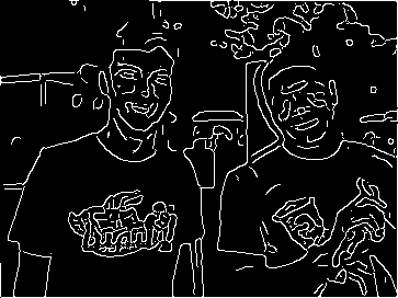
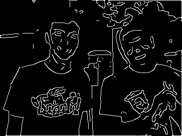
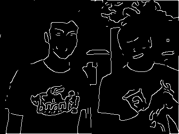
Note how there are fewer but more fluid edges for a larger filter width. This is because the noise is being filtered out, and more regions are blending together. Notice in particular how MJ's right arm is one fluid edge in the rightmost image for the larger gaussian width (also thanks to hysteresis thresholding that it's connected like that). One way to describe the progression from the image on the left to the image on the right is a sort of loss of fine detail, which is to be expected with more blurring. In other words, the sketch on the right is a rougher, more general sketch of MJ's outline. Hence, there is a tradeoff between filtering noise and retaining detail.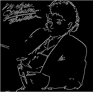
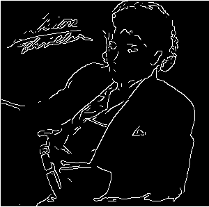
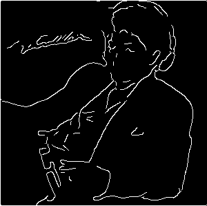
Command: Canny('mj.jpg', 0.5, 0, 0, 'mj_filter0.5')
(Using automatic thresholding)Command: Canny('mj.jpg', 1, 0, 0, 'mj_filter1')
(Using automatic thresholding)Command: Canny('mj.jpg', 2, 0, 0, 'mj_filter2')
(Using automatic thresholding) -
Varying the high threshold
In the following experiment, I will test the effect of varying the high threshold during the hysteresis thresholding stage, fixing sigma at 2 and the low threshold at 0.001 (remember that I normalized the image to [0, 1], so the high and low thresholds are also in this range since the gradient is in the range [0, 1])
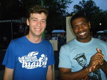
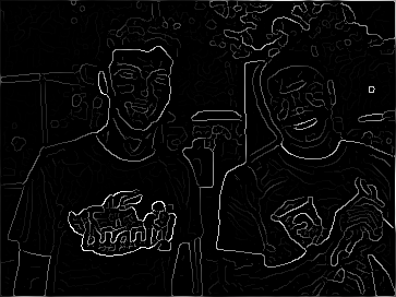
The input image The output of the nomaximum suppresion stage (does not change in any of the examples, since it is calculated before the hysteresis thresholding stage)
Command: Canny('reu.jpg', 2, 0.02, 0.001, 'reuth0.02') Command: Canny('reu.jpg', 2, 0.03, 0.001, 'reuth0.03') Command: Canny('reu.jpg', 2, 0.04, 0.001, 'reuth0.04'))
The results of this are consistent with the role of the high threshold, which is to ensure that at least one pixel in an edge of connected pixels exceeds a threshold. When I set that high threshold lower, more of the edges satisfy this criterion and are able to pass through tot he output image. Note the fine detail around the shoulders of Yohan's shirt that make it through when the high threshold is down at 0.02, versus how only the basic outline of the shirt is allowed to stay when the high threshold is 0.04. Overall, this has a similar effect to increasing sigma, however it does not change the output to nonmaximum suppression, so it has a higher chance of retaining finer detail (and it doesn't change the shape of any of the edges that pass through).
One other interesting point to note is that the edge that picks up the shadow behind Yohan's head is eliminated when transitioning from T_h=0.03 to T_h=0.04. This is an effect that would be hard to accomplish varying the other parameters.
Varying the low threshold
In the following experiment, I will test the effect of varying the low threshold during the hysteresis thresholding stage, fixing sigma at 1.5 and the high threshold at 0.05
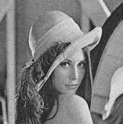
The input image The output of the nomaximum suppresion stage
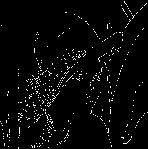
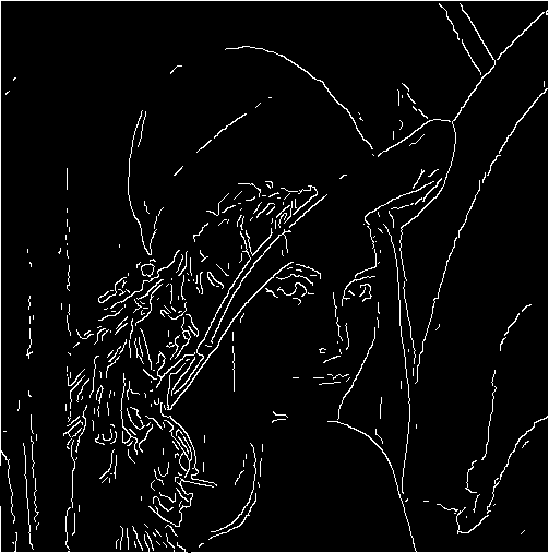
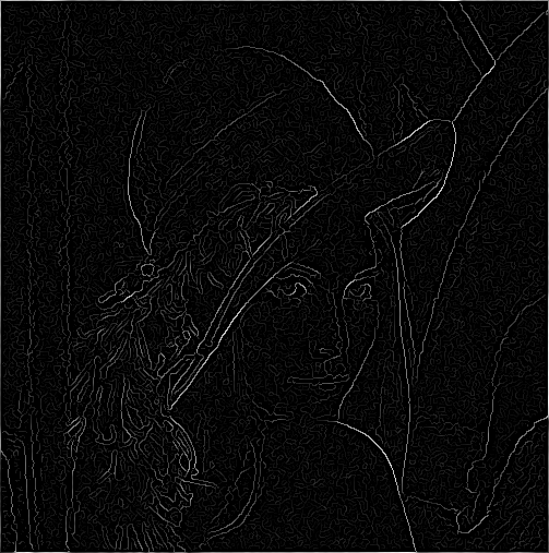
Command: Canny('lena.jpg', 1.5, 0.05, 0.05, 'lenatl0.05') Command: Canny('lena.jpg', 1.5, 0.05, 0.001, 'lenatl0.001')
In the first example, I set the low threshold equal to the high threshold, basically disabling the effect of hysteresis thresholding (if the low and high thresholds are equal, I'm not taking advantage of the dual thresholding capability). Notice how there are a lot of edges that are only 1 or two pixels wide, and the image looks broken up. In the second step, when I set the low threshold to 0.001 and allow pixels in the range [0.001, 0.05] to be connected together, I get much better results. Most of the 1-2 pixel wide edges have grown into longer edges, and the image looks better-connected. Look particularly around the nose and the outline of the hat.
Results on the given images
NOTE: I used my automatic thresholding to help find good values for T_h and T_l- The Mandrill
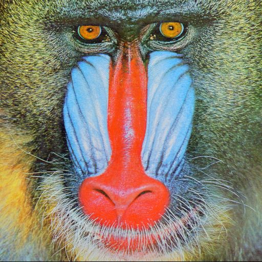
(sigma=1.5, T_h = 0.04, T_l = 0.001) 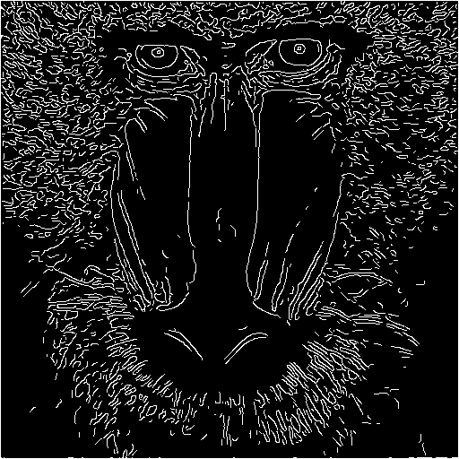
Command: Canny('mandrill.jpg', 1.5, 0.04, 0.001, 'mandrill_1') Notes: Trying generally to pick up some of the whiskers and the basic outline of the face
(sigma=4, T_h = 0.015, T_l = 0.001) 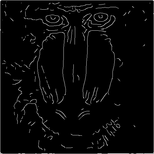
Command: Canny('mandrill.jpg', 4, 0.015, 0.001, 'mandrill_2') Notes: Increasing sigma to try to smooth out the whiskers a bit more so that only the general profile of the face is left
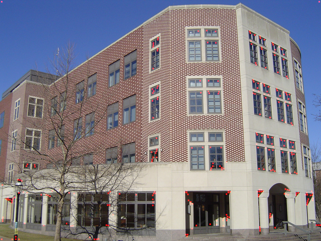
- The Computer Science Building at Princeton
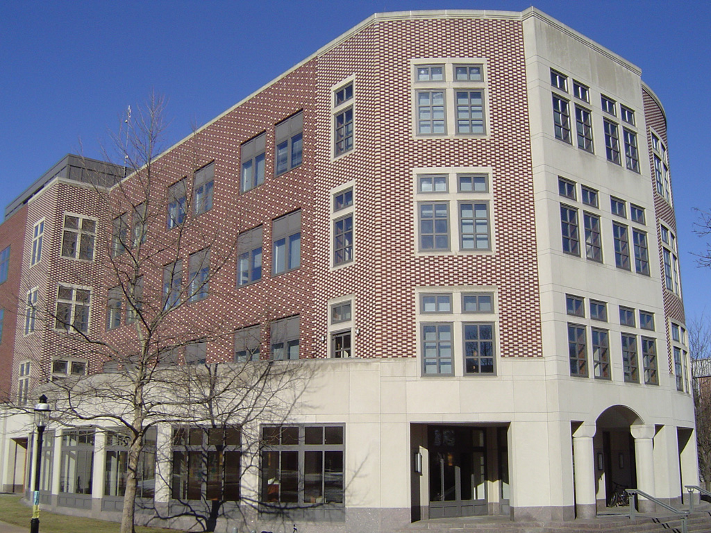
(sigma=0.5, T_h = 0.17, T_l = 0.002) 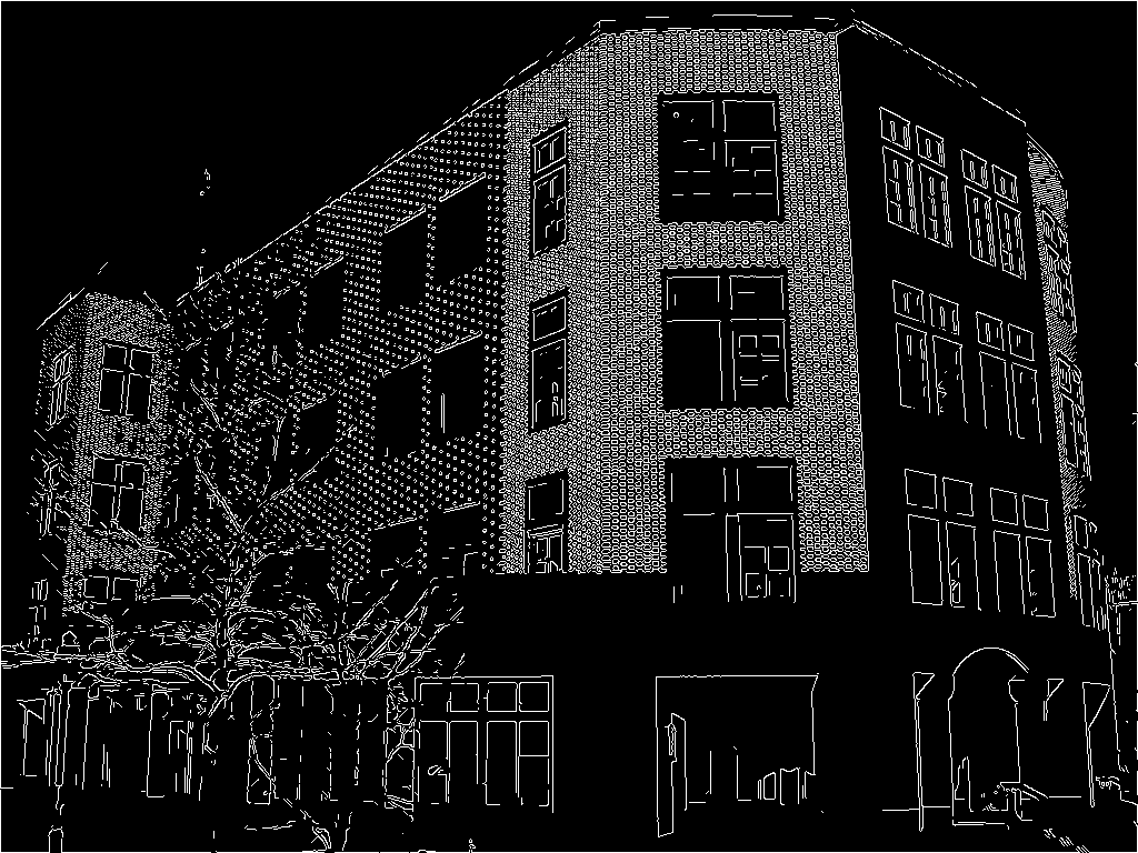
Command: Canny('csbldg.jpg', 0.5, 0.17, 0.002, 'cs_1'); Notes: Using a very small sigma so that the edges between individual bricks aren't blurred out
(sigma=2.5, T_h = 0.0214, T_l = 5e-5) 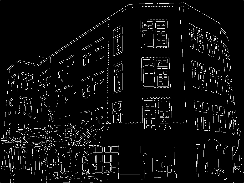
Command: Canny('csbldg.jpg', 2.5, 0.0214, 5e-5, 'cs_2'); Notes: Using a larger sigma to blur out the bricks and trying to get just the general outline of the building
Corner Detector (25%)
Algorithm Steps
- First find the filtered gradient, same as with the Canny Edge detector.
- If a region contains a corner, it will have a strong gradient in two distinct directions. but the directions are not necessarily orthogonal to the coordinate axes. To come up with a robust way to sense two strong gradient directions, define the following covariance matrix over the components of the gradient, Fx and Fy, in some sub-window of the image
\[ C = \left[ \begin{array}{cc} \sum Fx^2 & \sum FxFy \\ \sum FxFy & \sum Fy^2 \end{array} \right] \]
Since this matrix is symmetric, it will have all real eigenvalues and is similar to a diagonal matrix (whose coordinate axes will be in the direction of the two strongest gradient directions). It also turns out to be positive semi-definite (proof later), so it will always have two eigenvalues that are greater than or equal to zero. The eigenvalues each correspond to how strong each of the two strongest gradient directions are. So if we set a lower bound on how low the smallest eigenvalue is, we have enough information to say whether or not a corner exists in an area of an image.
In other words, to detect a corner, compute the matrix C as define above, and find its two eigenvalues. If the smallest eigenvalue is above some threshold, then assert that a corner exists there.
NOTE: Since that matrix has to be computed for every single point, it could take a very long time. To speed this up, I took advantage of Matlab's built-in, optimized convolution functions. That is, I created a 1D matrix of all 1s and convovled the original matrix with this twice, once in the vertical and once in the horizontal direction, for the matrices Fx*Fx, Fy*Fy, and Fx*Fy. This is the fastest way I could think of to compute those sums, and it scales well.
- Nonmaximum suppression: It is desirable to get rid of points that are marking the same corner, and to only store the strongest point for each corner. This is analogous to the thinning edge step in the Canny Edge Detector. After saving the points at which a corner is believed to exist, along with the smaller eigenvalue at that point, sort this list in descending order by the value of the small eigenvalue. Now go in order in the list. For each point, remove all points in the neighborhood of p that occur lower down in the list.
To speed this part up, I kept an extra matrix that stores the points believed to have their corners at their actual 2D locations. This helps to locate neighbor points quicker, since they are not in spatial order in the list sorted by eigenvalue
- The last step is to draw a red box around each corner area
- (Optional) Automatically determine the threshold of the eigenvalues (somewhere in step 2). My idea for this would be to take the average of all of the smallest eigenvalues and to set it to that, though I haven't had time to implement this idea so I don't know how well it works
Results Varing Parameters
There are three degrees of freedom in the corner detector: the width of the smoothed gradient filter (as before), the size of the rectangular neighborhood (in my program, I define this to be the distance from the center of a point to the edge of one of its neighbors), and the lower threshold for accepting something as a corner. The syntax for using my corner detector is as follow:Syntax: Corner(filein, sigma, Neighborhood size, Lower threshold, fileout)
Note that a whole neighborhood of pixels encompasses and area (2N + 1) x (2N + 1), where N is the "Neighborhood size" I defined above.
|
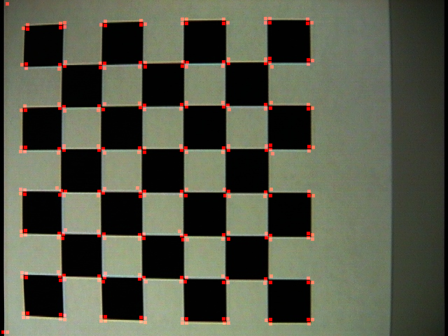 |
| Command: Corner('checker.jpg', 1, 5, 0.1, 'checker1.png') |
| Note: An initial run on this checkerboard (which has clear barrel distortion). Notice that it was able to find nearly every corner formed in this grid. Because I used a neighborhood of five, it got a response for |
|
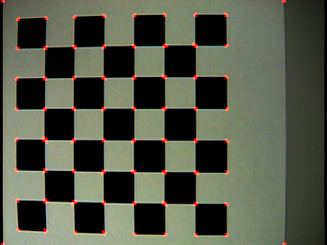 |
| Command: Corner('checker.jpg', 1, 2, 0.01, 'checker2.png') |
| Note: Here is the result of making the neighborhood smaller and trying to really hone in on the exact location of the corners. One problem with this is that the eigenvalues will be smaller (since the covariance matrices encompass a smaller region of the corner), so I had to lower the threshold from 0.1 to 0.01 for this to work. But I achieved my goal. |
|
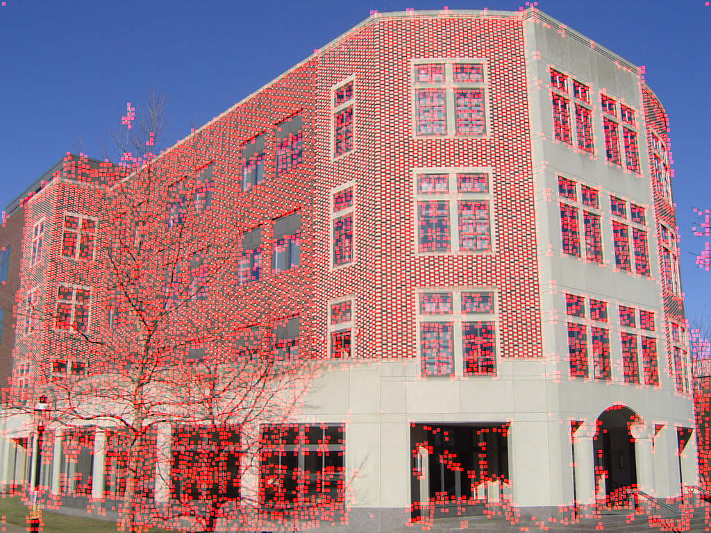 |
| Command: Corner('csbldg.jpg', 1, 5, 0.01, 'cornercs_1.png') |
| Here's a slightly tougher test case. Note that many of the little brick corners are being detected, which looks rather busy. |
|
 |
| Command: Corner('csbldg.jpg', 5, 5, 0.01, 'cornercs_2.png') |
| Here's an improved version showing how much of a difference varying sigma can make. I've chosen to make sigma much wider (5), to try to filter out the bricks. Now the corner detector safely ignores them and picks up on the building's other features a higher percentage of the time. NOTE that this is not perfect and still misses some corners, so thresholds sometimes need to be tweaked even more to get the desired results |
Scale Selection, AKA Blob Detector (25%)
The basic goal of the blob detector is to hone in on features in an image that may occur at different scales. Put simply, "how do I find lots all of the blobs in an image, given that they may be different sizes?" To help detect features, define some function that reaches its max value when it operates over a feature area. If a feature is defined as strong variations in the image gradient over many directions within a window, then a laplacian would be a good choice of such a function. But since the features can be different sizes, the laplacian should vary in width, and the size of the feature should be estimated to be the width of the laplacian that leads to the greatest output response.Algorithm Steps
- Approximate a noise-filtered laplacian by a difference of gaussians. For instance, the laplacian of width two would be approximated by a gaussian of width 2 minus a gaussian of width sqrt(2). Compute these differences of gaussians over the widths 1, sqrt(2), 2*sqrt(2), ... 32, and convolve each with the image. I figured a width of 32 would be as large as I needed; that leads to a gaussian that spans 2*(32)*3, or 192 pixels across 3 sigma on both sides. This is a huge blob.
- At each pixel in the image, find the width of the difference of gaussians (DOG) that lead to the greatest response. This is the global maximum over scale, and is the approximate size of a feature if it is present. To determine if a feature of that size is centered at the pixel in question, ensure that the response at that scale is a local maximum over the 26 pixels around it in space.
Note the reason that the global maximum in scale is taken, is to prevent concentric squares from being drawn around the same point. The highest response should be over the scale that fits the image the tightest. This is because a smaller square would be inside the blob where the gradient varies little, and the larger square would not fit the blob as tightly and would have a smaller response (since a wider gaussian gets scaled down in height). This is a picture of the case to prevent:
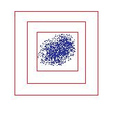
Only the inner-most square should be kept - Draw a red square around the blob with a width equal to the width of the DOG that gave the greatest response.
Results of the Blob Detector
Syntax: ScaleSelection(filein, threshold, fileout)
where threshold is the lower bound on the response from the DOG that's counted as a feature
| ||
| ||
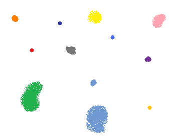
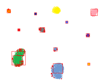
| Command: ScaleSelection('blobs.png', 0.1, 'blobout.png'); | ||
| Note that these results are pretty good; it drew a square of the correct size for all blobs but one (it missed the yellow blob at the top somehow). Note how there is at most one square centered at a point (the result for choosing the global maximum over scale per pixel). Note also how in addition to some of the "big squares" that make a tight fit to different sections of the blobs, there are also a few little squares around the edges and around single pixel fringes of the spraypaint blobs. This is because an edge and a single pixel blob is still a feature, it just wouldn't have as big of a response for a larger DOG (it takes up a higher percentage of the area for a smaller filter). One more cool effect to point out is in the green blob which bends a little bit, there's one square that fits most of it, and another two squares that fit the top and bottom sections of it. So the blob detector was sophisticated enough to recognize that both as one continuous feature that has two smaller sections making it up. |
| ||
| ||
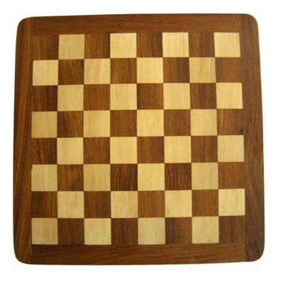
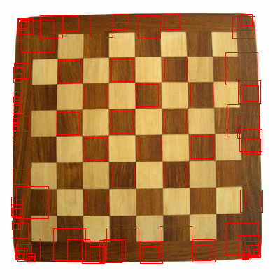
| Command: ScaleSelection('chessboard.jpg', 0.07, 'chessblob.png'); | ||
| Note how the program was able to correctly figure out the size of the chessboard cells and to locate most of them towards the center. It was thrown off a bit towards the border since techically, there's more variation there. |
| ||
| ||
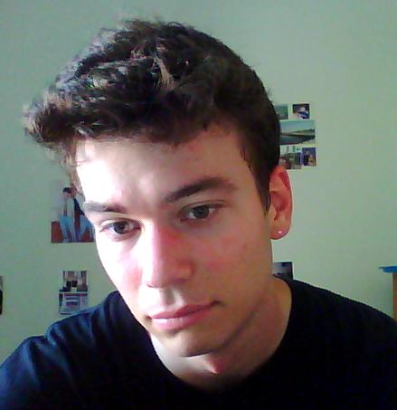
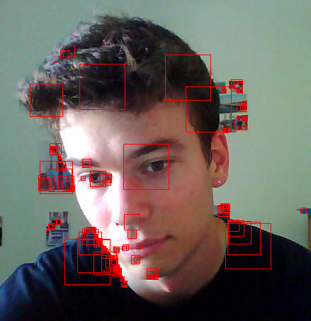
| Command: ScaleSelection('myface.jpg', 0.05, 'faceblob.png'); | ||
| Here are some of the features of my face :-). Note how it sort of got my eyes, which is the main reason I wanted to try this out (because I hear that eye tracking is a difficult problem...and this looks like evidence of that fact). It also got parts of my hair (I was having a bad hair day), the top of my nose, part of the contours of my lips, and my chin. Also, it apparently really liked the sharp edges from my shoulders. I'm glad to see it actually missed my Adam's apple, which tends to protrude a bit more than I'd like to admit. |
Code Summary
blog comments powered by Disqus